Logo image

Section A.1 Civil Engineering: Trusses and Struts

Subsection A.1.1 Activities

Definition A.1.1.

In engineering, a truss is a structure designed from several beams of material called struts, assembled to behave as a single object.
described in detail following the image
A photograph of a bridge, with the steel girders forming triangles.
Figure 65. A simple truss
described in detail following the image
A diagram representing a simple truss. Points are labeled A,B,C,D,E, with A and B on the same level on top, and C,D, and E below. The truss is represented by three adjacent triangles: ACD, ADB, and BDE. Below points C and E are small blue triangles, representing where the bridge is anchored to the ground. A red arrow points downward from D in the middle of the truss, representing the load put on the truss.
Figure 66. A simple truss

Activity A.1.2.

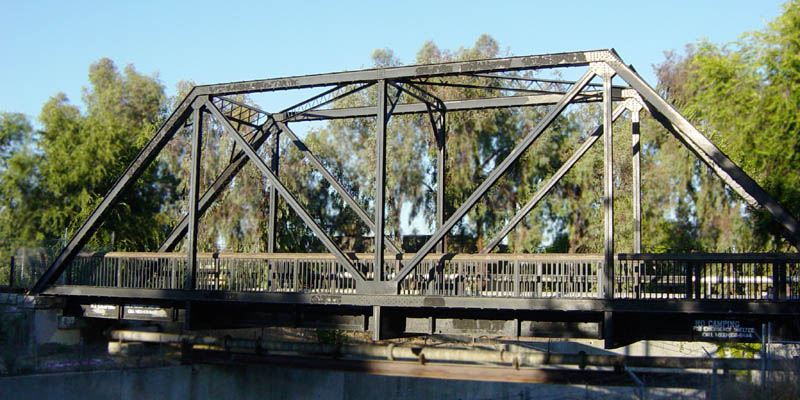
Consider the representation of a simple truss pictured below. All of the seven struts are of equal length, affixed to two anchor points applying a normal force to nodes \(C\) and \(E\text{,}\) and with a \(10000 N\) load applied to the node given by \(D\text{.}\)
described in detail following the image
The simple truss in FigureΒ 66 is reproduced.
Figure 67. A simple truss
Which of the following must hold for the truss to be stable?
  1. All of the struts will experience compression.
  2. All of the struts will experience tension.
  3. Some of the struts will be compressed, but others will be tensioned.

Observation A.1.3.

Since the forces must balance at each node for the truss to be stable, some of the struts will be compressed, while others will be tensioned.
described in detail following the image
The simple truss in FigureΒ 66 is reproduced, but with additional decorations. A blue arrow points up and to the right from C, and up and to the left from E. Edges AB, AC and BE are decorated with red double sided outward arrows indicating tension. Edges AD and BD are decorated with red double sided inward arrows indicating compression.
Figure 68. Completed truss
By finding vector equations that must hold at each node, we may determine many of the forces at play.

Remark A.1.4.

For example, at the bottom left node, 3 forces are acting.
described in detail following the image
The simple truss in FigureΒ 66 is reproduced, but with additional decorations. At C, red arrows point parallel to the struts towards A and D. A blue arrow points up and to the right from C.
Figure 69. Truss with forces
Let \(\vec F_{CA}\) be the force on \(C\) given by the compression/tension of the strut \(CA\text{,}\) let \(\vec F_{CD}\) be defined similarly, and let \(\vec N_C\) be the normal force of the anchor point on \(C\text{.}\)
For the truss to be stable, we must have:
\begin{equation*} \vec F_{CA}+\vec F_{CD}+\vec N_C=\vec 0 \end{equation*}

Activity A.1.5.

Using the conventions of the previous remark, and where \(\vec L\) represents the load vector on node \(D\text{,}\) find four more vector equations that must be satisfied for each of the other four nodes of the truss.
described in detail following the image
The simple truss in FigureΒ 66 is reproduced.
Figure 70. A simple truss
\begin{equation*} A: \unknown \end{equation*}
\begin{equation*} B: \unknown \end{equation*}
\begin{equation*} C: \vec F_{CA}+\vec F_{CD}+\vec N_C=\vec 0 \end{equation*}
\begin{equation*} D:\unknown \end{equation*}
\begin{equation*} E:\unknown \end{equation*}

Remark A.1.6.

The five vector equations may be written as follows.
\begin{equation*} A: \vec F_{AC}+\vec F_{AD}+\vec F_{AB}=\vec 0 \end{equation*}
\begin{equation*} B: \vec F_{BA}+\vec F_{BD}+\vec F_{BE}=\vec 0 \end{equation*}
\begin{equation*} C: \vec F_{CA}+\vec F_{CD}+\vec N_C=\vec 0 \end{equation*}
\begin{equation*} D: \vec F_{DC}+\vec F_{DA}+\vec F_{DB} +\vec F_{DE}+\vec L=\vec 0 \end{equation*}
\begin{equation*} E: \vec F_{EB}+\vec F_{ED}+\vec N_E=\vec 0 \end{equation*}

Observation A.1.7.

Each vector has a vertical and horizontal component, so it may be treated as a vector in \(\IR^2\text{.}\) Note that \(\vec F_{CA}\) must have the same magnitude (but opposite direction) as \(\vec F_{AC}\text{.}\)
\begin{equation*} \vec{F}_{CA} = x\begin{bmatrix} \cos(60^\circ) \\ \sin(60^\circ) \end{bmatrix} = x\begin{bmatrix} 1/2 \\ \sqrt{3}/2\end{bmatrix} \end{equation*}
\begin{equation*} \vec{F}_{AC} = x\begin{bmatrix} \cos(-120^\circ) \\ \sin(-120^\circ) \end{bmatrix} = x\begin{bmatrix} -1/2 \\ -\sqrt{3}/2\end{bmatrix} \end{equation*}

Activity A.1.8.

To write a linear system that models the truss under consideration with constant load \(10000\) newtons, how many scalar variables will be required?
  • \(7\text{:}\) \(5\) from the nodes, \(2\) from the anchors
  • \(9\text{:}\) \(7\) from the struts, \(2\) from the anchors
  • \(11\text{:}\) \(7\) from the struts, \(4\) from the anchors
  • \(12\text{:}\) \(7\) from the struts, \(4\) from the anchors, \(1\) from the load
  • \(13\text{:}\) \(5\) from the nodes, \(7\) from the struts, \(1\) from the load
described in detail following the image
The simple truss in FigureΒ 66 is reproduced.
Figure 71. A simple truss

Observation A.1.9.

Since the angles for each strut are known, one variable may be used to represent each.
described in detail following the image
The simple truss in FigureΒ 66 is reproduced, but now each strut is labeled with a variable. Struts AB, AC, AD, BD, BE, CD, and DE are labeled \(x_1, \ldots, x_7\) respectively.
Figure 72. Variables for the truss
For example:
\begin{equation*} \vec F_{AB}=-\vec F_{BA}=x_1\begin{bmatrix}\cos(0)\\\sin(0)\end{bmatrix} =x_1\begin{bmatrix}1\\0\end{bmatrix} \end{equation*}
\begin{equation*} \vec F_{BE}=-\vec F_{EB}=x_5\begin{bmatrix}\cos(-60^\circ)\\\sin(-60^\circ)\end{bmatrix} =x_5\begin{bmatrix}1/2\\-\sqrt{3}/2\end{bmatrix} \end{equation*}

Observation A.1.10.

Since the angle of the normal forces for each anchor point is unknown, two variables may be used to represent each.
described in detail following the image
The simple truss in FigureΒ 66 is reproduced, but with additional decorations. Blue arrows representing normal forces point up and to the right from C, and up and to the left from E.
Figure 73. Truss with normal forces
\begin{equation*} \vec N_C=\begin{bmatrix}y_1\\y_2\end{bmatrix} \hspace{3em} \vec N_D=\begin{bmatrix}z_1\\z_2\end{bmatrix} \end{equation*}
The load vector is constant.
\begin{equation*} \vec L = \begin{bmatrix}0\\-10000\end{bmatrix} \end{equation*}

Remark A.1.11.

Each of the five vector equations found previously represent two linear equations: one for the horizontal component and one for the vertical.
described in detail following the image
The simple truss in FigureΒ 66 is reproduced, with the variables labeling each strut.
Figure 74. Variables for the truss
\begin{equation*} C: \vec F_{CA}+\vec F_{CD}+\vec N_C=\vec 0 \end{equation*}
\begin{equation*} \Leftrightarrow x_2\begin{bmatrix}\cos(60^\circ)\\\sin(60^\circ)\end{bmatrix}+ x_6\begin{bmatrix}\cos(0^\circ)\\\sin(0^\circ)\end{bmatrix}+ \begin{bmatrix}y_1\\y_2\end{bmatrix}=\begin{bmatrix}0\\0\end{bmatrix} \end{equation*}
Using the approximation \(\sqrt{3}/2\approx 0.866\text{,}\) we have
\begin{equation*} \Leftrightarrow x_2\begin{bmatrix}0.5\\0.866\end{bmatrix}+ x_6\begin{bmatrix}1\\0\end{bmatrix}+ y_1\begin{bmatrix}1\\0\end{bmatrix}+ y_2\begin{bmatrix}0\\1\end{bmatrix}= \begin{bmatrix}0\\0\end{bmatrix} \end{equation*}

Activity A.1.12.

Expand the vector equation given below using sine and cosine of appropriate angles, then compute each component (approximating \(\sqrt{3}/2\approx 0.866\)).
described in detail following the image
The simple truss in FigureΒ 66 is reproduced, with the variables labeling each strut.
Figure 75. Variables for the truss
\begin{equation*} D:\vec F_{DA}+\vec F_{DB}+\vec F_{DC}+\vec F_{DE}=-\vec L \end{equation*}
\begin{equation*} \Leftrightarrow x_3\begin{bmatrix}\cos(\unknown)\\\sin(\unknown)\end{bmatrix}+ x_4\begin{bmatrix}\cos(\unknown)\\\sin(\unknown)\end{bmatrix}+ x_6\begin{bmatrix}\cos(\unknown)\\\sin(\unknown)\end{bmatrix}+ x_7\begin{bmatrix}\cos(\unknown)\\\sin(\unknown)\end{bmatrix}= \begin{bmatrix}\unknown\\\unknown\end{bmatrix} \end{equation*}
\begin{equation*} \Leftrightarrow x_3\begin{bmatrix}\unknown\\\unknown\end{bmatrix}+ x_4\begin{bmatrix}\unknown\\\unknown\end{bmatrix}+ x_6\begin{bmatrix}\unknown\\\unknown\end{bmatrix}+ x_7\begin{bmatrix}\unknown\\\unknown\end{bmatrix}= \begin{bmatrix}\unknown\\\unknown\end{bmatrix} \end{equation*}

Observation A.1.13.

The full augmented matrix given by the ten equations in this linear system is shown below, where the eleven columns correspond to \(x_1,\dots,x_7,y_1,y_2,z_1,z_2\text{,}\) and the ten rows correspond to the horizontal and vertical components of the forces acting at \(A,\dots,E\text{.}\)
\begin{equation*} \left[\begin{array}{ccccccccccc|c} 1&-0.5&0.5&0&0&0&0&0&0&0&0&0\\ 0&-0.866&-0.866&0&0&0&0&0&0&0&0&0\\ -1&0&0&-0.5&0.5&0&0&0&0&0&0&0\\ 0&0&0&-0.866&-0.866&0&0&0&0&0&0&0\\ 0&0.5&0&0&0&1&0&1&0&0&0&0\\ 0&0.866&0&0&0&0&0&0&1&0&0&0\\ 0&0&-0.5&0.5&0&-1&1&0&0&0&0&0\\ 0&0&0.866&0.866&0&0&0&0&0&0&0&10000\\ 0&0&0&0&-0.5&0&-1&0&0&1&0&0\\ 0&0&0&0&0.866&0&0&0&0&0&1&0\\ \end{array}\right] \end{equation*}

Observation A.1.14.

This matrix row-reduces to the following.
\begin{equation*} \sim \left[\begin{array}{ccccccccccc|c} 1&0&0&0&0&0&0&0&0&0&0&-5773.7\\ 0&1&0&0&0&0&0&0&0&0&0&-5773.7\\ 0&0&1&0&0&0&0&0&0&0&0&5773.7\\ 0&0&0&1&0&0&0&0&0&0&0&5773.7\\ 0&0&0&0&1&0&0&0&0&0&0&-5773.7\\ 0&0&0&0&0&1&0&0&0&-1&0&2886.8\\ 0&0&0&0&0&0&1&0&0&-1&0&2886.8\\ 0&0&0&0&0&0&0&1&0&1&0&0\\ 0&0&0&0&0&0&0&0&1&0&0&5000\\ 0&0&0&0&0&0&0&0&0&0&1&5000\\ \end{array}\right] \end{equation*}

Observation A.1.15.

Thus we know the truss must satisfy the following conditions.
\begin{align*} x_1=x_2=x_5&=-5882.4\\ x_3=x_4&=5882.4\\ x_6=x_7&=2886.8+z_1\\ y_1&=-z_1\\ y_2=z_2&=5000 \end{align*}
In particular, the negative \(x_1,x_2,x_5\) represent tension (forces pointing into the nodes), and the positive \(x_3,x_4\) represent compression (forces pointing out of the nodes). The vertical normal forces \(y_2+z_2\) counteract the \(10000\) load.
described in detail following the image
The simple truss in FigureΒ 66 is reproduced, with the red decorations indicationg tension on struts AC, AB, and BE and compression on struts AD and BD. The blue normal force vectors pointing up and right from C and up and left from E are also shown.
Figure 76. Completed truss